Conjugate of piecewise function
In this post, we’ll show how to calculate the conjugate of a piecewise function  ,
,
such as

The conjugate for the above is:

where  is the conjugate of the function
  constrained to
  . So, computing the conjugate of a piecewise function is simple as long as the conjugates of the sub-functions can be computed easily.
Conjugate of constrained function
In this section, we’ll show how to calculate the convex conjugate of a function  , which is the function which is constrained to a domain
  .
.
The conjugate is defined as:

For the unconstrained case, the solution would be given by:
![\begin{align*} x = \left[f' \right]^{-1}(y), \end{align*}](http://www.mcduplessis.com/wp-content/ql-cache/quicklatex.com-55aae9701945aa634e3dbd13ca3b1209_l3.png "Rendered by QuickLaTeX.com")
where  is the derivative of . Since is convex, is a monotonically increasing function. Therefore, we have

The conjugate of the constrained function is therefore:

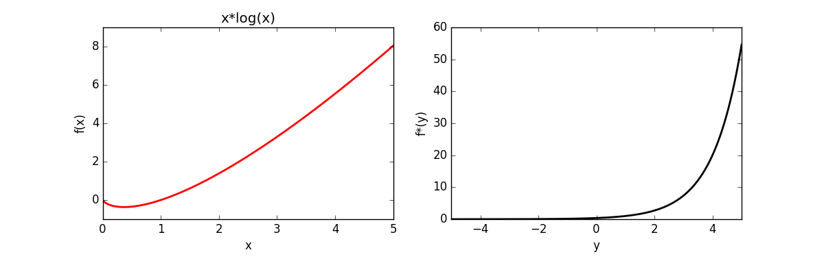
The convex conjugate for the unconstrained function can be automatically calculated in Python — as described in the previous post.
Code that do the above is given below:
def calc_const_conj(fun_str, lstr='l', ustr='u', varnames='x l u', fname='plot.png'):
    # set the symbols
    vars = sp.symbols(varnames)
    x = vars[0] if isinstance(vars, tuple) else vars
    y = sp.symbols('y', real=True)

    # set the function and objective
    fun = parse_expr(fun_str)
    obj = x*y - fun
    fun_diff = sp.diff(fun, x)
    obj_diff = sp.diff(obj, x)

    l = parse_expr(lstr)
    u = parse_expr(ustr)

    # calculate yl and yu
    yl = sp.simplify(fun.subs(x, l))
    yu = sp.simplify(fun.subs(x, u))

    dyl = sp.simplify(fun_diff.subs(x, l))
    dyu = sp.simplify(fun_diff.subs(x, u))

    # calculate derivative of obj and solve for zero
    sol = solve(obj_diff, x)

    # substitute solution into objective
    solfun = sp.collect(sp.simplify(obj.subs(x, sol[0])), x)

    # print the function and conjugate:
    print('{0:45} y < {1}'.format(str(sp.simplify(l*y - yl)), dyl))
    print('{0:45} {1} <= y <= {2}'.format(str(solfun), dyl, dyu))
    print('{0:45} y > {1}'.format(str(sp.simplify(u*y - yu)), dyu))

# Example: calc_const_conj('1/2*x**2', lstr='-1', ustr='1', varnames='x')
Table of conjugates
| Function | Constraint | Conjugate | ||
| Linear |  |
|
 |
|
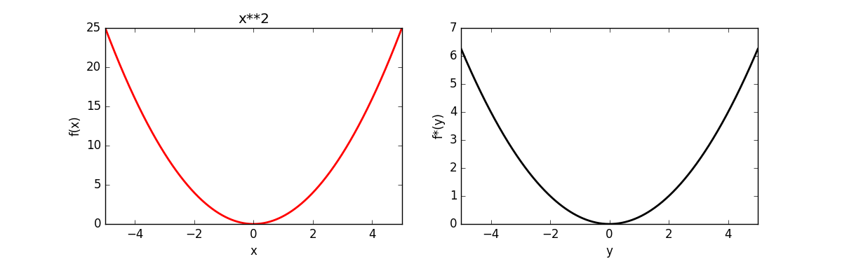
| Simple Quadratic |  |
|
 |
|
| Quadratic |  |
|
 |
|
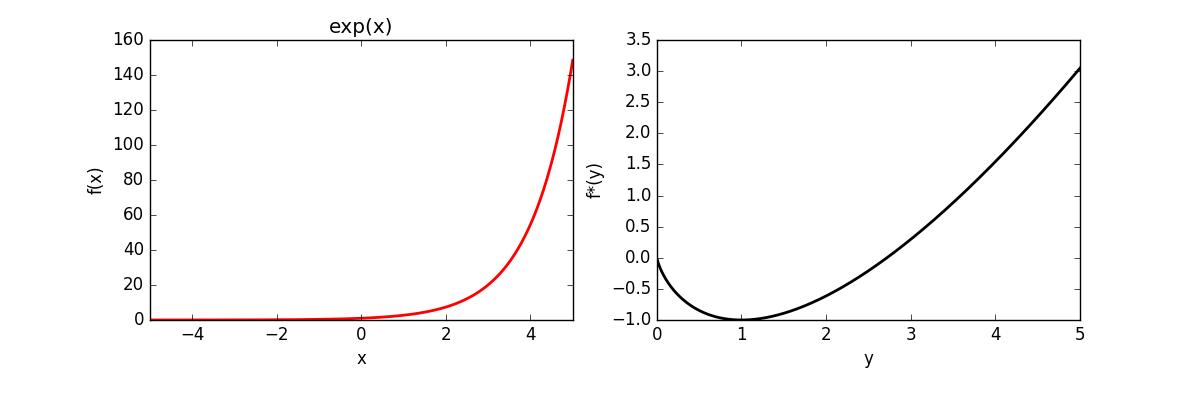
| PE-like |  |
 |

|
|
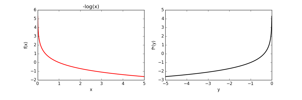
| Hinge |  |
 |
||
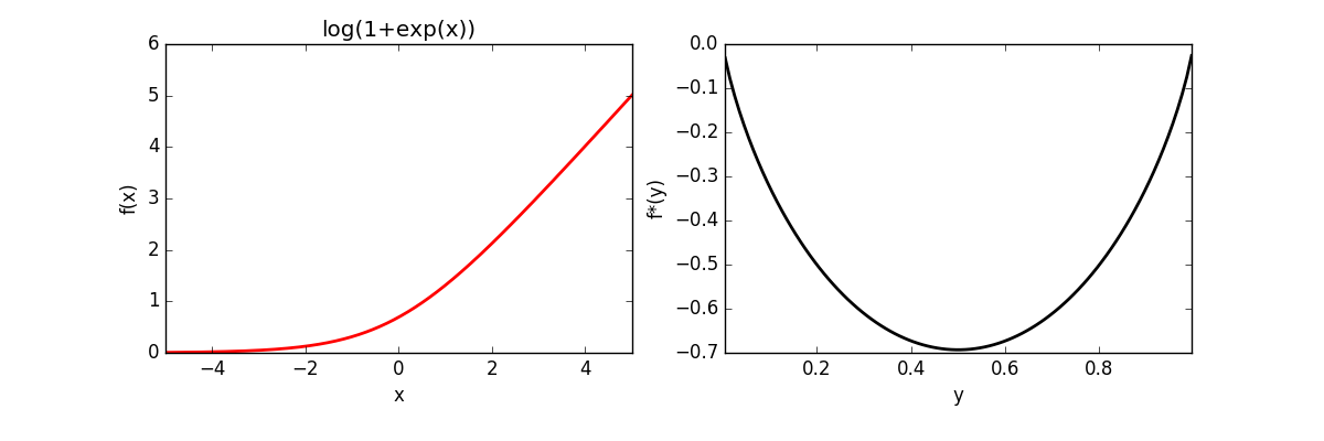
| (scaled)Hinge |  |
|


![[1-y]\log(1-y) + y\log y](http://www.mcduplessis.com/wp-content/ql-cache/quicklatex.com-092fd768096949889799505b8500bda4_l3.png "Rendered by QuickLaTeX.com")


 , we mean the solution to the following optimization problem:
 . The objective function that we wish to solve is:
![\begin{align*} L(\lambda) & = \min_{x} \sum_{i=1}^{n}\left[\frac{1}{2}(x_i - y_i)^2 + \lambda a_i x_i \right] -\lambda\qquad \textrm{s.t.} \quad x \succeq 0, \\ & =\min_{x} \sum_{i=1}^{n}\left[\frac{1}{2}x_i^2 - x_i[y_i - \lambda a_i]- \frac{1}{2}y_i^2\right] - \lambda \qquad \textrm{s.t.} \quad x \succeq 0. \end{align*}](http://www.mcduplessis.com/wp-content/ql-cache/quicklatex.com-ec69243cdbdcd49401aaa472a9e2eaa1_l3.png "Rendered by QuickLaTeX.com")
 decouples (for fixed
  ) it can be solved as:

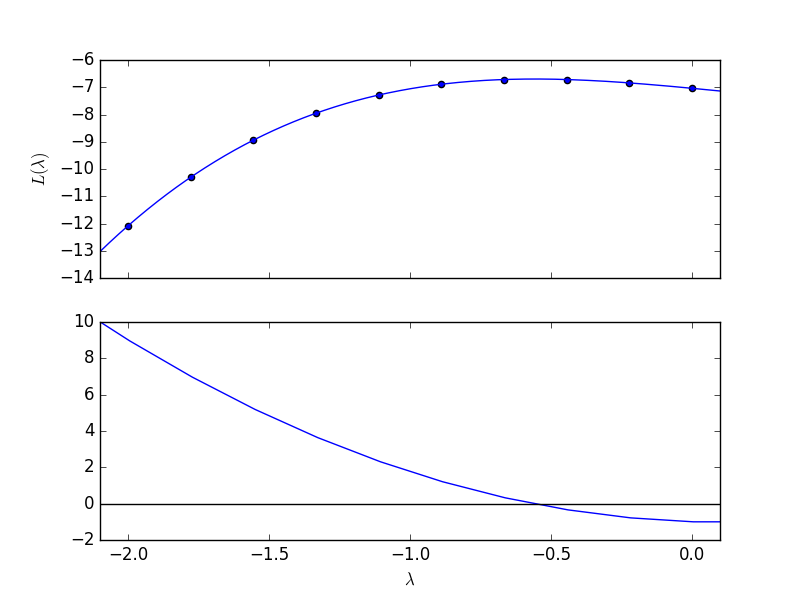
 . To determine where the variables will switch on we sort the values according to
  .
. that sorts according to

 , so that


 , but
, but  .
.
 = x^2")